Essential tips for exporting and cleaning data with Spark

I often receive various requests from customers while working on FastTrack projects, and I have compiled some examples to help you build your solution on top of a data lake using useful tips. Most of the examples in this post use pandas, and I hope they will be helpful for you as they were for me.

Please note that all examples in this post use pyspark.

In my scenario, I exported multiple tables from SQLDB to a folder using a notebook and ran the requests in parallel.

In this post, we will discuss the logic of reusing the same session mentioned here at MSSparkUtils is the Swiss Army knife inside Synapse Spark. I will show comments made by my colleague martinB in more detail in the next example, which explains how to export data from SQLDB into the data lake.

Exporting the data and building the lab

from concurrent.futures import ThreadPoolExecutor timeout = 3600 # 3600 seconds = 1 hour notebooks = [ {"path": "notebook1", "params": {"param1": "value1"}}, {"path": "notebook2", "params": {"param2": "value2"}}, {"path": "notebook3", "params": {"param3": "value3"}}, ] with ThreadPoolExecutor() as ec: for notebook in notebooks: ec.submit(mssparkutils.notebook.run, notebook["path"], timeout, notebook["params"])

If you're looking to use a thread pool for launching parallel tasks, you can refer to the documentation on concurrent.futures — Launching parallel tasks — Python 3.11.1

You may also want to check out Microsoft's Synapse Spark pool optimization framework, which can help improve your logical execution on Spark. This framework is available through multiple notebooks on the same cluster instance.

For the script we'll be discussing, we'll create a notebook called "Notebook_interactive". This notebook will connect to the Adventureworks2017 database hosted on the SQLDB server using a SQL Server user through the JDBC connector. The table names will be parameters that will be input into this notebook through another one that will trigger the parallel execution. The data will be exported to my storage connected to Synapse on the following path: "/SQLDB_intrc/Tables/".

Notebook_interactive code:

#set variable to be used to connect the database database = "AdventureWorks2017" table = parameterString user = "USERHERE" password = "PASSWORDHERE" #print(nametable.value ) jdbcDF = spark.read \ .format("jdbc") \ .option("url", f"jdbc:sqlserver://SERVERNAME.database.windows.net:1433; database=AdventureWorks2017") \ .option("dbtable", table) \ .option("user", user) \ .option("password", password).load() jdbcDF.write.mode("overwrite").parquet("/SQLDB_intrc/Tables/" + parameterString )

To demonstrate the use of a thread pool, I will provide a brief example with the table names Production.Product and Production.Workorder hardcoded into a notebook. This notebook will be used to trigger the parallel execution.

from concurrent.futures import ThreadPoolExecutor timeout = 1800 #seconds notebooks = [ {"path": "/Notebook_interactive", "params": {"parameterString":"Production.Product"}}, {"path": "/Notebook_interactive", "params": {"parameterString":"Production.WorkOrder"}} ] with ThreadPoolExecutor() as ec: for notebook in notebooks: ec.submit(mssparkutils.notebook.run, notebook["path"], timeout, notebook["params"])

As you can see in Fig 1 - execution, it shows both notebooks were called and executed in parallel:

Fig 1 - execution

Ok. Data is now exported, now let's work on it!

Organizing the data

If you're not familiar with terms such as Data Lake, Lakehouse, Bronze, Silver, and Gold, it would be helpful to learn more about them. Here are some references to get started:

Assuming you've read the above content or you're already familiar with it, let's dive into how to handle the exported data.

The data is typically landed in the Bronze or Raw zone. From there, we can move it to the Silver zone where we can clean and organize it for our analytics project, which will connect to the Gold zone.

Please note that all examples in this post will use PySpark.

Cleaning the Data

Now, let's move on to some tips on how to clean your data. The techniques you choose to use will depend on your specific business requirements.

We'll start with an example using the Production.Product file. In the following examples, we'll be using pandas to visualize the data, so we'll start by using the head() method to open and review the file in different formats:

1) CSV with pandas

import pandas as pd ##CSV df = pd.read_csv(r'https://StorageAccount.blob.core.windows.net/Container/FILENAME.csv') #shows the data df.head()

2) Excel - For this, you will need to install the xlrd package.

You can install it by running the following command in a notebook cell:

!pip install xlrd

Reading the excel file:

import pandas as pd file =('https://StorageAccount.blob.core.windows.net/Container/filename.xlsx') excel_panda = pd.read_excel(file) ##show the data read from the excel spreadsheet excel_panda.head()

3) Parquet - For parquet, we will use a slightest different approach.

There are multiple ways to read an Excel file in Synapse Analytics. One approach is to use pandas as mentioned in the documentation: Tutorial: Use Pandas to read/write ADLS data in serverless Apache Spark pool in Synapse Analytics

Another approach is to copy the file locally using mssparkutils and then read it from there.

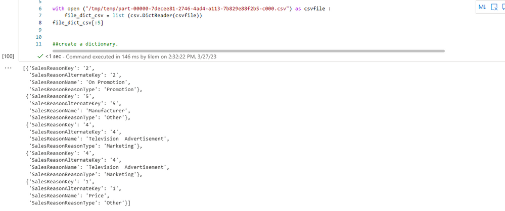
import pandas as pd mssparkutils.fs.cp('/SQLDB_intrc/Tables_introc/Production.Product/FILENAME.snappy.parquet', 'file:/tmp/temp/FILENAME.parquet') pf = pd.read_parquet('file:/tmp/temp/FILENAME.parquet') pf.head()

If you prefer to use "with open" to handle files, you can still use the same approach to read and write files in ADLS. Here's an example of reading a CSV file using "with open" and creating a dictionary:

import csv #mssparkutils.fs.cp('/folderonthestorage/filename.csv', 'file:/tmp/temp/filename.csv') with open ("/tmp/temp/filename.csv") as csvfile : file_dict_csv = list (csv.DictReader(csvfile)) #showing first 5 file_dict_csv[:5]

Fig 2 - Dictionary, shows what I just mentioned.

The dictionary will "create an object that operates like a regular reader but maps the information in each row to a dict whose keys are given by the optional fieldnames parameter." ref: csv — CSV File Reading and Writing — Python 3.11.2 documentation

Fig 2 - Dictionary

This is the File that was just read for the dictionary creation. Refer to Fig 3 - File, for the results:

Fig 3 - File.

Great, now that you have the data, you can proceed to filter it and measure the time taken.

Filtering

Continuing from where we left off, my Product file exported from AdventureWorks.

Hence, another question arises: how can we measure the fastest approach?

Let's suppose I want to filter the SafetyStockLevel columns from the data frame. I want values that are greater than 700 and smaller than 1100. How can I do that? Well, there are some different approaches. Generally, the best is the one that gives me accurate results as fastest as possible.

Let's now explore two different approaches for filtering the SafetyStockLevel column of the data frame, where we want to keep values greater than 700 and smaller than 1100. The best approach is generally the one that provides accurate results as quickly as possible.

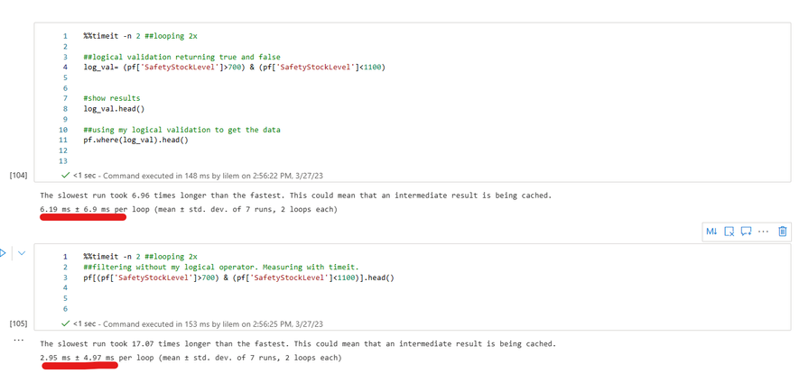
For the filter, I will show you 2 different approaches, to measure the speed of these approaches, we will use the timeit function.

1) Filtering approach 1 - It will create a boolean mask that will return true or false(log_val). That mask will be used to filter the data frame (pf) that contains data for Product.

Filtering Approach 1: We create a boolean mask that returns true or false (log_val) based on the condition we want to filter. This mask is then used to filter the data frame (pf) that contains data for the Product table.

##logical validation returning true and false ##pf stands for the dataframe that was used to read the data from the parquet file. #so pf here is jsut a dataframe name log_val= (pf['SafetyStockLevel']>700) & (pf['SafetyStockLevel']<1100) ##using my logical validation to get the data pf.where(log_val).head()

Filtering approach 2: Directly filter the data frame using the predicate.

pf[(pf['SafetyStockLevel']>700) & (pf['SafetyStockLevel']<1100)].head()

The second approach appears faster to me since it is more straightforward. However, to confirm this, I will use timeit.

First, create a notebook cell and run the following:

import timeit

Now, let's use timeit by referencing it with %%timeit and loop it 2 times. Fig 4 - timeit, will show the results:

Fig 4 - timeit

Alright, the second approach has been shown to be faster!

NaN, NA and null values

NaN stands for not a number, as NA represents a missing value. Null represents an empty object. There are different ways to handle this, using pandas NaN, NA and Null values would sometimes be handled with the same methods.

Following are some examples:

isna

"Return a boolean same-sized object indicating if the values are NA. NA values, such as None or numpy.NaN, gets mapped to True values. "

Note: pf on the example is a data frame with Production data.

import pandas as pd pd.isna(pf)

ref:pandas.DataFrame.isna — pandas 1.5.3 documentation (pydata.org)

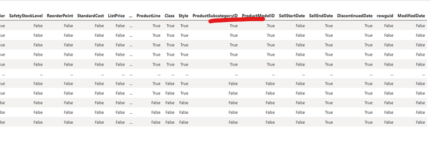
Fig 5 - isna, shows the results for isna execution. As you can see a boolean mask was created returning true or false:

Fig 5 - isna

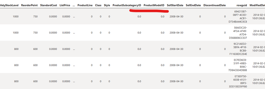
Fillna can be used to replace the values and handle NA, NaN . In this example, I am replacing it with zero. Per documentation "Fill NA/NaN values using the specified method."

Note: pf on the example is a data frame with Production data.

import pandas pf=pf.fillna(0,inplace=True) pf.head()

ref: pandas.DataFrame.fillna — pandas 1.5.3 documentation (pydata.org)

Fig 6 - fillna, shows the results. So as you can see values that were returned as true by isna are now replaced by zero using fillna:

Fig 6 - fillna

Null

"Detect missing values.

Return a boolean same-sized object indicating if the values are NA. NA values, such as None or numpy.NaN, gets mapped to True values. Everything else gets mapped to False values. "

Note: pf on the example is a data frame with Production data

import pandas Log_val = pf.isnull() Log_val.head()

ref: pandas.DataFrame.isnull — pandas 1.5.3 documentation (pydata.org)

Results on Fig 7 - isnull, shows a boolean mask:

Fig 7 isnull

Not Null

It is possible also to do the opposite, instead of using isnull() use notnull(). Not null will return true for not null values. So, also returns a boolean mask for Not Null values.

Log_val = pf.notnull() Log_val.head()

Replacing values

Now, null, NaN values were handled. My requirements for cleaning this data should cover replacing values. There are different ways to replace values inside the data frame. I will show a few examples of replacing numbers and strings with pandas and regex.

Replace string

The following examples demonstrate how to search for a string and replace it in the data frame.

As mentioned previously, the data frame in the example below is represented by pf. The code will search for the word "headset" in the Name column of the data frame(pf) and if there is an exact string match (case-sensitive), it will be replaced by "HeadSt".

import pandas as pd #Replace "headset" with "HeadSt" pf['Name'] = pf['Name'].str.replace(r"headset", "HeadSt")

If you need to change the text of a column to lowercase. In this case, let's use as an example the column Name, you could use the following code.

pf['Name'] = pf['Name'].str.lower()

Follow another example using regex to replace the value in a case-insensitive way.

import pandas as pd import re # Use regex to replace "headset" with "HeadSt" pf['Name'] = pf['Name'].str.replace(re.compile(r"headset", re.IGNORECASE), "HeadSt")

Replace numbers

This is a very simple example that shows how to replace values in a column:

To replace the values that are equal to 750 with 800 in the "Reorderpoint" column for the dataframe "pf", you can use the following code:

pf['ReorderPoint']= pf['ReorderPoint'].replace([750],800)

New column

Ok. So let's now create a new column, one of my requirements is to create a column as a result of a calculation. Hence, I will import the data of the file "Production.WorkOrder" into data frame df and subtract EndDate from StartDate. My new column will be named Order_days.

import pandas as pd mssparkutils.fs.cp('/SQLDB/Tables/Production.WorkOrder/file.parquet', 'file:/tmp/temp/file.parquet') df = pd.read_parquet('/tmp/temp/file.parquet') df.head() ##new column was created by subtracting the end date from the End date and start date df['Order_days'] = df['EndDate'] - df['StartDate']

Merge

My final requirement is to merge Dataframes. Therefore, I will merge the "pf" data frame containing product data and the "df" data frame containing work orders. This will be done through a left join using "productid" as the key, and a new data frame will be created from the resulting merge.

import pandas as pd #on = the columns name newpf= pd.merge (pf,df, how='left',on ='ProductID') newpf.head()

Summary

My intention here is to share some useful tips for data cleaning during the Silver Zone before moving to the Gold Zone. In this regard, I have provided examples using Python/Pandas that demonstrate opening files with different formats, creating a dictionary from a CSV file, handling NaN, NA, and Null values, filtering data, creating new columns, and merging data frames.

Liliam, UK

Learn more